Wikipedia’s articles graph analysis

Introduction

During this analysis we would work with Wikipedia' graph, witch I recollected following the instructions and techniques of Complex Network Analysis in Python-Pragmatic Bookshelf, when I mined the network, I structured the graph as a directed network. However to facilitate the analysis, I read the edge list as an undirected graph, then we could say, originally it was a directed graph, but for this work, we will work it as an undirected network.

Network Characteristics

Network Basic Parameters

Number of nodes (N) represent the number of components in the system, for this analysis our net had 3656 nodes, there are 3656 edges in the network.

what do nodes represent?

Nodes represent Articles in Wikipedia.

What do links represent?

links represent the connection between two articles.

Do links have direction?

In the begin yes, they do. However for this analysis we will analyze it, as a undirected graph (without direction)

Do links have weights?

Every connection has a weight of 1

Now, the graph density measures the fraction of existing edges out of all potentially possible edges and the network density’s 0.002

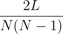
We could calculate using for undirected networks. The density of the Wikipedia network is low, only about 0.1 percent. Only two out of about 1,000 possible edges exists in the graph.

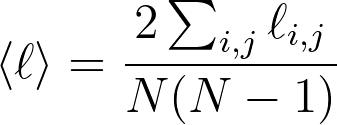
Other interesting measure is the Average Path Length, witch is obtained by the next function we got an average distance of 2.96.

It is not possible to see the data clearly, so they are presented in text, since there are only 4 different distances.

{1: 14915, 2: 993243, 3: 4918899, 4: 754283}

Now for the eccentricity we got these data.

{3: 571, 4: 3084, 2: 1}

Now using the last information we could say that radius (of a graph) is 2 and the diameter is 4.

Periphery (of a graph) this is a little complicate, because this metric is a set for this network we got 3084 in the set, then for this reason instead of listed the nodes, we could see an image.

Center (of a graph) at different of the last measure this set only content the node {‘Complex Network’}

One reason to work this network as undirected is because the clustering is undefined for directed graphs, the clustering coefficient is the fraction of possible triangles that contain the ego node and exist and the measure for the network is 0.695.

According to Complex Network Analysis in Python-Pragmatic.

“If the clustering coefficient of a node is 1, the node participates in every possible triangle involving any pair of its neighbors; the egocentric network of such a node is a complete graph. If the clustering coefficient of a node is 0, no two nodes in the neighborhood are connected; the egocentric network of such node is a star.”

Summary

Centrality Measure

The simplest centrality measure is a node degree (also indegree and outdegree, when you can use them). Intuitively, a node with more edges, representing, say, an article with more ties, is more important than other node with less ties, in other words, a node with a high degree centrality may be capable of affecting a lot of neighbors in its neighborhood at once, but we cannot say anything about the opportunities for global outreach. The minimum and maximum degree centrality are 0.0005 and 0.160, respectively.

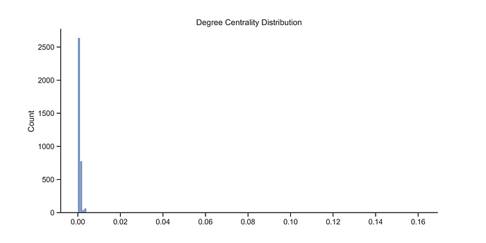
Other important centrality measure is the closeness centrality, because using this measure we could obtain the reciprocal mean distance (length of the geodesics) from a node to all other reachable nodes in the network. This show us how close the node in to the rest of the graph. Just like the last measure (Degree Centrality) this measure is in the range from 0 (for nodes who don’s have neighbors) to 1 the node is the hub of the global network and it has a path to any other node.

Degree Distribution and Models of Networks.

We need set some assumptions, first the node’s grade is equivalent to his relevance in the network, also we assume the top nodes with biggest grade are the most important node in a subgraph generated of a community detection.

To improve the image, we could plot a range in the image using the quantiles, in this case we could use 0.05 and 0.95.

Top 10 nodes:

('Social Network', 586),
('Doi (Identifier)', 544),
('Isbn (Identifier)', 513),
('Issn (Identifier)', 481),
('Computer Network', 373),
('Small-World Network', 373),
('Network Science', 364),
('World Wide Web', 347),
('Artificial Neural Network', 344),
('Random Graph', 344)

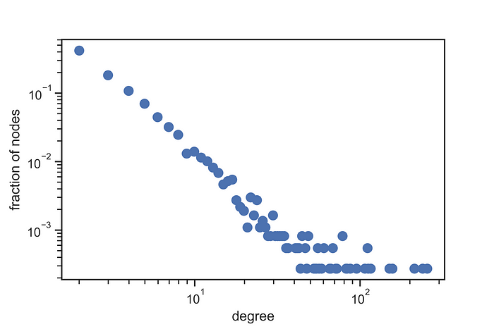
Now, maybe is a little complicated observe the information in the histogram and the list, particularity by the results, in the case of the histogram there are 202 nodes with a degree of 11. However not is possible identify them and in other hand the list only show a little part of the information. For try to improve the information’ compression we could see the next graph where we could identify that the farthest nodes are smaller than the closer nodes and using this graph we could refuse our second assumption, “we assume the top nodes with biggest grade are the most important node in a subgraph generated of a community detection.”, because some of this nodes are in a closed distance and maybe not is the optimal node for a future communities detection.

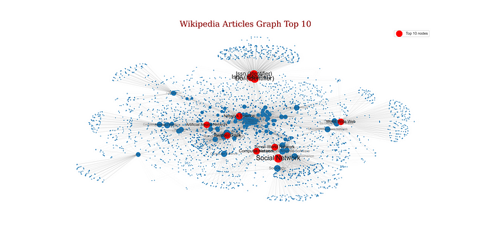
After of analyze the network, the node with highest degree is the article ‘Social Network’ with a degree of 586, and the lowest article is ‘Bianconi–Barabási Model’ with a degree of 2.

from distribution’ behavior we could think it is a scale-free network or an exponential network, then we need find gamma to recreate the behavior in a synthetic network.

For any case, We could clearance the last formulas to obtain gamma, the reason to use those functions, it is because we have the Kmin and the Kmax, moreover we know N, after of replace the respective values, and resolve each formula, we got gamma for a exponential network is 0.01404, and for a scale-free network could be 2.44434. I choice form the network as scalar-free network, consequently we could see the next distributions.

Community Detection

Once we know most of the attributes of the network, the next step was to identify what type of clusterization to apply to the graph, always remembering that the modularity had to have a good score so that we can relay.

What I used was the greedy modularity community, this because at the network characteristics I had the opportunity to see the distribution of the graph, and it was likely to have more than 2 clusters, that is the reason why I did not use the Neuman’s algorithm. Once I made the cluster, with the help Of Networkx, 8 different communities were identified. And it made a lot of sense, the clusters where clear segmentations, and the communities generated corresponded to the visualization.

Once I had the visualization from intuition I expected to have a high score in modularity, nevertheless in order to have more backup I got the score so that I can evaluate my graph the best way, the results were stunning, I personally believe that I was going to have between .3 and .4, but after the calculation the modularity score was of .52, which is tell us that the detection of the communities was successfully accomplished.

References

[1] Dmitry Zinoviev — Complex Network Analysis in Python-Pragmatic (2018)

[2] Gjermëni, Orgeta. (2015). POWER LAW DISTRIBUTION AS A COMPONENT OF THE VERTEX DEGREE DISTRIBUTION ON A SOCIAL UNIVERSITY NETWORK COURSE. European Scientific Journal, ESJ. 11. 1857–7881.

[3] McAuley, J., 2021. Learning to Discover Social Circles in Ego Networks. [online] I.stanford.edu. Available at: [Accessed 23 June 2021].

[4] Albert-Laszlo Barabasi — Network Science-Cambridge University Press (2016)